General linear model in Python and C

The goal of this post is to explain how to use general linear model in Python and C. It is assumed that the reader has basic understanding of the regression inference.

Introduction

Why are we using Python and C in this example? Python code is often said to be an “executable pseudocode”, i.e., Python syntax is relatively easy to read and comprehend. On the other hand, C programming language is the foundation modern computing, and alongside Fortran still plays an important role in parallel computing. This post in a prerequisite for parallelization of fitting a large number of general linear models for hundreds of data values per each model.

For readers less familiar with the regression model and linear least squares formulation, please refer to this linear least squares example and an example on ordinary least squares (OLS) with modelling a non-linear relationship. Polish speaking reader is redirected to the materials I once prepared for cognitive science students. OLS assumes homoscedasticity of the errors, i.e., all variables are assumed to have the same, finite variance. Note using in this example data on average heights and weights for American women aged 30–39, from The World Almanac and Book of Facts, 1975.

Another important distinction is between a linear regression model with one independent variable (X) explaining one dependent variable (Y). It can be formulated mathematically as:

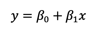
where:
    * y — dependent variable;
    * β₀ — intercept of the regression line;
    * β₁ — slope of the regression line.

The notation I use is similar to the one used by prof. Michael Lacey from the Yale University, e.g., here.

In more general terms, the relationship between multiple (n) regressors (independent variables) and a dependent variable can be modeled as:

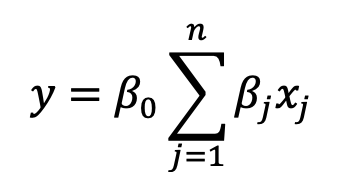
where:
    * y — dependent variable;
    * β₀ — intercept of the regression line;
    * n — number of the explanatory variables (parameters of the regression line to be fit);
    * β_j — parameters of the regression line;
    * x_j — explanatory variables;

See also materials from prof. Lacey’s course on statistics, topic: Multiple Linear Regression.

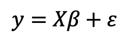
Matrix representation of the multiple linear regression is:

Additionally, algebraic form of the ordinary least squares problem is:

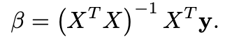
as nicely explained by Frank, Fabregat-Traver, and Bientinesi (2016; available on arxiv).

OLS was implemented in most modern programming languages (see these Rosseta Code examples), including Python and C. Note also that the linked Python and C examples are a bit misleading, as there are is in fact an example with quadratic fitting utilized there (see ordinary least squares example mentioned above).

Python

The Python example I prepared in Jupyter Notebook is available below. Please note, the same data are consistently used: heights and weights for American women (see this explanation).

In order to understand how to use this implementation for calculating multiple linear regression (linear, with more than one dependent variable), please consider the following example:

Hence, the presented implementation works well in all of the following cases:

• One dependent variable, linear fitting
• One dependent variable, quadratic fitting
• More than one dependent variable, linear fitting

---

C

As mentioned above, multiple regression is also implemented in C programming language (see this example). The modified example, using stock exchange data is:

#include <stdio.h>
#include <gsl/gsl_matrix.h>
#include <gsl/gsl_math.h>
#include <gsl/gsl_multifit.h>

/* Interest rate */
double r[] = { 2.75, 2.5, 2.5, 2.5, 2.5, 2.5, 2.5, 2.25,
               2.25, 2.25, 2,2, 2, 1.75, 1.75, 1.75, 1.75,
               1.75, 1.75, 1.75, 1.75, 1.75, 1.75, 1.75 };
/* Unemployment rate */
double u[] = { 5.3, 5.3, 5.3, 5.3, 5.4, 5.6, 5.5, 5.5,
               5.5, 5.6, 5.7, 5.9, 6, 5.9, 5.8, 6.1,
               6.2, 6.1, 6.1, 6.1, 5.9, 6.2, 6.2, 6.1 };
/* Stock index price */
double s[] = { 1464, 1394, 1357, 1293, 1256, 1254, 1234,
               1195, 1159, 1167, 1130, 1075, 1047, 965, 943,
               958, 971, 949, 884, 866, 876, 822, 704, 719 };

int main()
{
	int n = sizeof(r)/sizeof(double);
	gsl_matrix *X = gsl_matrix_calloc(n, 3);
	gsl_vector *Y = gsl_vector_alloc(n);
	gsl_vector *beta = gsl_vector_alloc(3);

	for (int i = 0; i < n; i++) {
		gsl_vector_set(Y, i, s[i]);

		gsl_matrix_set(X, i, 0, 1);
		gsl_matrix_set(X, i, 1, r[i]);
		gsl_matrix_set(X, i, 2, u[i]);
	}

	double chisq;
	gsl_matrix *cov = gsl_matrix_alloc(3, 3);
	gsl_multifit_linear_workspace * wspc = gsl_multifit_linear_alloc(n, 3);
	gsl_multifit_linear(X, Y, beta, cov, &chisq, wspc);

	printf("Beta:");
	for (int i = 0; i < 3; i++)
		printf("  %g", gsl_vector_get(beta, i));
	printf("\n");

	gsl_matrix_free(X);
	gsl_matrix_free(cov);
	gsl_vector_free(Y);
	gsl_vector_free(beta);
	gsl_multifit_linear_free(wspc);
}

See this code also as gist: https://gist.github.com/mikbuch/d87c34489b20f170405827a5fccdcf06#file-ols_linear_multiple_regression-c

Compile and run C code example:

$gcc -Wall ols_linear_multiple_regression.c -lgsl -o ols_linear_multiple_regression.o && 
./ols_linear_multiple_regression.o

Expected output:

Beta: 1798.4 345.54 -250.147

Summary

To sum up, in this post presented basic usage of general linear model’s implementation in Python and C. Future steps are to: (i) implement parallel GLM fitting, e.g., for multiple models being calculated at the same time; and (ii) use some real-world data, e.g., neuroimaging data.

Bibliography

Frank, A., Fabregat-Traver, D., & Bientinesi, P. (2016). Large-scale linear regression: Development of high-performance routines. Applied Mathematics and Computation, 275, 411-421.